Sargassum landfall alert at J+3: detection, advection, and confidence level

Detection: isolating high floating-algae-index pixels

The entry point is a Copernicus Marine satellite product: a floating-algae proxy index, akin to NFAI (Normalized Floating Algae Index), computed pixel by pixel over the Guadeloupe area. Rather than fixing an absolute density threshold — fragile against day-to-day variability in observation conditions — the system applies a quantile threshold on that day's distribution: the 0.95 quantile by default, meaning pixels within the top 5% of intensity in the image.

This choice has a direct, deliberate consequence: the quantile threshold adapts to each scene rather than to a fixed physical value. If the 0.95 quantile fails to isolate valid pixels on a given image — too much cloud cover, too little signal — the system falls back through more permissive quantiles (0.90, then 0.85, then 0.80) until it obtains a usable set. This is an operational-robustness trade-off, not a scientific refinement: a degraded detection is preferable to no detection at all.

The retained pixels form the candidate patches — the starting points for the advection simulation. No biomass or volume estimate is derived from them: the product tells you where relative density is high, not how much sargassum is physically present.

Advection: where do these patches go over three days?

Once candidate patches are identified, each is represented by a set of virtual particles. These particles are integrated forward in time through the Copernicus Marine surface current field (u, v components), over a J+3 horizon. This is first-order Lagrangian advection: transport follows the surface current directly, with no Stokes drift, no wind drag, and no fragmentation model for the patches.

To avoid producing a single trajectory — deceptively precise — the system runs several members in parallel (ten by default). Each member applies a small perturbation: an initial spatial offset and noise added to the current field. The goal is not to simulate alternative weather scenarios, but to surface a transport uncertainty envelope — the spread across members then becomes a data point used at the next step.

Zone impact: p_mean, hit_rate, and ETA

The Guadeloupe coastline is divided into predefined coastal zones. For each zone and each ensemble member, the system tests the intersection between the advected trajectory and the zone polygon. From this per-member binary test, three quantities are computed:

p_mean

The average, across all ensemble members, of the per-member impact probability — the fraction of members reaching the zone.

hit_rate

The proportion of members whose probability of reaching the zone is strictly positive — how many members, out of ten, reach the zone at all, regardless of intensity.

ETA per member / median ETA

Estimated arrival time for each member that reaches the zone; the median across those members is retained as the zone's ETA. With no impact, no ETA is computed.

p_mean is not a volumetric probability — how much sargassum will arrive — but a transport probability metric: the fraction of simulated trajectories that actually reach the zone. This is a distinction that simulation-based coastal forecasting systems generally share: the model tells you where transport leads, not how much quantity gets there.

The confidence logic: why p_mean alone is not enough

This is the most important point in the system, and the one that separates a usable alert from a plain probability chart. A high p_mean produced by a large majority of members converging on the same zone at the same time is not worth the same as an identical p_mean produced by a mix of widely dispersed members — some reaching the zone at J+1, others at J+3, others not at all. The average can be identical; the reliability of the information is not.

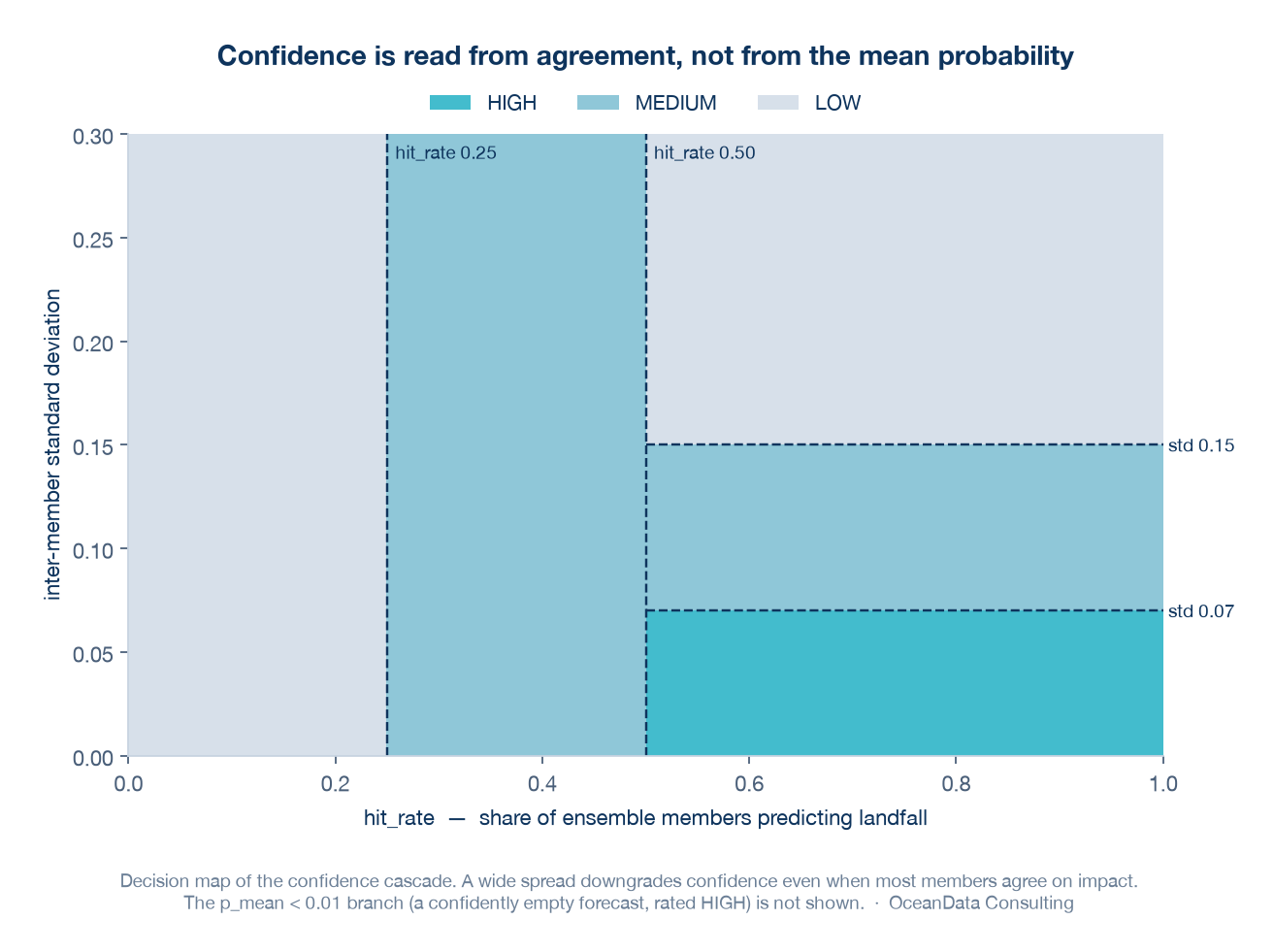
The system therefore does not average away the uncertainty: it classifies it explicitly, from the pair (hit_rate, inter-member standard deviation), following a cascade of rules:

• p_mean < 0.01 → HIGH confidence (the signal is weak and consistent: every member agrees there is no impact)
• hit_rate < 0.25 → LOW confidence (too few members reach the zone to draw a conclusion)
• hit_rate < 0.50 → MEDIUM confidence (a minority of members converge, without a clear majority)
• hit_rate ≥ 0.50, then on the standard deviation of probabilities across members: std < 0.07 → HIGH; std < 0.15 → MEDIUM; otherwise → LOW

This last branch carries the core message: even when a majority of members agree on impact (hit_rate ≥ 0.50), the system downgrades confidence to LOW if the inter-member spread remains wide (standard deviation ≥ 0.15). A high p_mean built on a fragile agreement between members is flagged as such, rather than presented with the same assurance as a high p_mean built on a tight agreement. Confidence is therefore never a function of p_mean alone — it measures the consistency of the ensemble, not just its center.

What this MVP does not do

It is worth being precise about the scope of this system, because that precision is what makes it usable for what it actually is — a coastal proof of concept — rather than for what it is not.

• No field validation: no coastal observation campaign has yet confronted the generated alerts against an actual landfall event. No detection rate, no accuracy score, no performance statistic can therefore be cited — nothing is measured at this stage.
• Transport is first-order only: no Stokes drift, no wind drag, no fragmentation model, and no biological decay of the patches. This is a transport approximation, not a sargassum life-cycle model.
• No data assimilation and no in-situ observational correction — the system ingests Copernicus products as-is and propagates them forward.
• Satellite product latency is a real, explicitly tracked operational constraint: an observation timestamp and its data-availability (generation) date do not coincide. An NFAI product dated today may have been generated with a lag of several hours, which bounds how fresh a J+3 alert actually is — an alert issued from an observation that is already hours old loses that much of its useful horizon.
• Geographic scope is limited to Guadeloupe and a predefined set of coastal zones: no automatic generalization to other islands.

The system's outputs — a JSON file, PNG probability and confidence maps, an optional PDF report — are designed to support a human decision, not to replace one. A transport-only alert system with an explicit confidence logic is a defensible foundation for discussing an operational deployment; it is not one yet.

Working on a coastal alert or forecasting system and want to discuss a confidence method suited to your case? Get in touch.

Sources and references

The metrics, comparisons and maps specific to this article are OceanData Consulting results and calculations; the links below document the datasets, standards and publications used.

• Copernicus Marine — ocean colour and floating algae products
• Copernicus Marine — global ocean physics analysis and forecast (surface currents)

Frequently asked questions

Related articles