
By Matthieu Caillaud · Founder, oceanographer
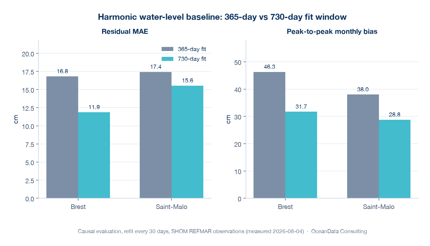
How long a record should a harmonic water-level baseline be fitted on? The usual answer — “a year, because that is a full cycle” — is precisely the wrong one, for a reason that can be established before any measurement: 365 days fall exactly on the Rayleigh threshold of the annual constituent Sa. Measured causally on 2026-08-04, moving from a 365-day to a 730-day fit window cuts the residual MAE by 29 % at Brest (16.82 → 11.87 cm) and by 11 % at Saint-Malo (17.44 → 15.55 cm). What follows explains why, and why that fit depth ended up deciding a verdict everyone assumed belonged to the model.
Fit depth is not a setting, it is a separability constraint
A harmonic analysis decomposes the observed water level into constituents of known frequency. Two constituents of neighbouring frequencies can only be separated if the fit window is at least as long as their beat period: that is the Rayleigh criterion. This is not a numerical preference but an identifiability limit — below it, the fit no longer distinguishes the two lines and splits the energy between them arbitrarily.
Three thresholds shape the choice of window for a tide gauge on the Atlantic-Channel coast:
- 90 days
- Separates neither S2/K2 nor K1/P1: 182.6 days are required for each of those pairs. The window does not carry Sa either.
- 365 days
- Separates S2/K2 and K1/P1, but falls exactly on the Rayleigh threshold of the annual constituent Sa: it is therefore estimated at the edge of its separability — noisy, and poorly extrapolated at every refit.
- 730 days
- Two rolling years. Sa is separated with margin, the estimate stops being marginal, and extrapolation between refits degrades far more slowly.
The 365-day case is the treacherous one, because it looks correct. A full year does “contain” an annual cycle, and the fit returns a perfectly plausible Sa amplitude. What is missing is not the signal but the margin: a constituent estimated exactly at its separability threshold is estimated at maximum variance, and that variance later surfaces as a slow drift of the predicted mean level.
The causal measurement: three years of observations, one variable
A separability argument is not a measurement. The question was therefore settled on 2026-08-04 by causal comparison on the scoreboard’s two water-level stations, Brest and Saint-Malo (SHOM REFMAR observations): three years of observations, the same evaluation window — the last 365 days —, a refit every 30 days in both arms, and a single variable changing, the fit depth.
“Causal” is the operative word here: every prediction is produced only from constants fitted on observations predating the target date. A non-causal two-year fit leaves a residual at 13.3 cm standard deviation — but that figure cannot be served, since it uses the future.
- Brest — 365 d
- Residual MAE 16.82 cm, standard deviation 20.77 cm, peak-to-peak monthly bias 46.3 cm.
- Brest — 730 d
- Residual MAE 11.87 cm, standard deviation 15.57 cm, peak-to-peak monthly bias 31.7 cm.
- Saint-Malo — 365 d
- Residual MAE 17.44 cm, standard deviation 22.21 cm, peak-to-peak monthly bias 38.0 cm.
- Saint-Malo — 730 d
- Residual MAE 15.55 cm, standard deviation 19.89 cm, peak-to-peak monthly bias 28.8 cm.
That is 29 % less MAE at Brest and 11 % less at Saint-Malo, causally, with no leakage. The secondary result is just as useful: the non-causal ceiling of 13.3 cm standard deviation was therefore mostly a matter of window depth rather than information leakage — the causal 730-day fit, at 15.57 cm standard deviation on Brest, comes close to it. In other words, most of what looked lost by refusing to see the future is recovered simply by looking further into the past.
The least spectacular column of that table is the one that sets up the next section: peak-to-peak monthly bias. At 365 days, the Brest baseline wanders across 46.3 cm of monthly bias amplitude over the evaluation year. That is not noise, it is drift — and drift can be corrected.
The unexpected effect: a better baseline did not narrow the AI model’s margin
The metocean AI scoreboard compares a post-processing model against the official baseline every day, and a quality gate withholds any station where the model fails to beat its own baseline on the training data. For that comparison to be fair, the gate does not pit the model against the raw baseline but against a debiased baseline: the baseline’s mean bias over the window is removed before the comparison. That is the correct methodological reflex — penalising a competitor for a constant offset would be a straw man.
The reflex backfires the moment the baseline drifts. As long as the harmonic baseline drifted by ±20 cm a month, the gate’s debiased baseline could remove 7.8 cm of bias for free over the test month — a correction no operational service could ever apply in advance, since it assumes knowing the bias of the very month being forecast. The AI model was therefore facing an artificially strong opponent, and drew against it: −0.2 % skill excluding bias.
With the baseline conditioned on two years, that bias falls to 0.4 cm: there is no longer anything substantial to remove for free, and the model’s real skill appears — +8.0 % on the same comparison. The model did not change. The opponent stopped being advantaged.
The methodological corollary is worth stating plainly, because it is not specific to tides: a model that fails against a biased baseline has not been measured, it has been compared to an artefact. The conclusion holds in both directions. A gain published against a drifting baseline is just as uninterpretable, except that it flatters instead of penalising.
What fit depth changed in the published verdict
The trajectory of the verdicts, station by station, shows how much the fit depth was driving publication:
- At a 90-day fit, both Brest and Saint-Malo sat below the gate.
- At 365 days, on a one-month test window, Brest passed at +7.97 % skill excluding bias and Saint-Malo failed at +4.95 %, 0.05 point short of the threshold.
- As of 2026-08-04, both stations clear the gate (gate.json: +53.25 % and +30.16 %, weak: false), bringing the scoreboard to 8 published stations.
Attribution has to be precise here, otherwise this article would tell a false story in the other direction. The figures published on 2026-08-04 are not the effect of the harmonic window alone: they combine the 730-day baseline, a training forcing stratified by run age, and the addition of tidal phase and pressure tendency as features (Brest +53.9 % excluding bias, 11.8 → 5.4 cm MAE; Saint-Malo +34.1 %, 15.1 → 9.9 cm). The effect attributable to the 365 → 730 day change alone is the table in the previous section, on the baseline itself. Both statements are true; they answer different questions.
A third factor, unrelated to the baseline, was fixed in the same pass: the test window was 30 days long, hence the very month of retraining. On the Atlantic-Channel coast, storm surge is a winter phenomenon, and the measurement confirms it — Brest’s residual MAE is 7.1 cm in July, 10.9 cm across all seasons, and 21.2 cm at the February 2026 peak. A verdict issued in July and one issued in November are not comparable. The test window for water-level stations was therefore extended to a full year.
A drifting baseline makes every feature ablation uninterpretable
The costliest consequence of this story is not a verdict, it is a measurement that had to be discarded. Mean sea-level pressure had been dropped from the features on 2026-08-03, after measurement. That measurement was made against the short harmonic baseline — the drifting one. But a seasonal drift and a pressure signal are both low-frequency phenomena: in that regime they are inseparable, and the ablation was not measuring what it believed it was measuring. Re-measured against the 730-day baseline, mean sea-level pressure is worth +17 points of skill excluding bias at Brest. It was reinstated, on water-level stations only — the wave and wind paths remain without pressure, where it cost 1 to 5 points, and where a wave height has no inverse-barometer response anyway.
Hence a sequencing rule that is anything but anecdotal: no new feature is measured against a baseline that is itself changing, and improving the physical baseline comes before adding capacity to the model. An ablation run against a baseline known to be about to improve by 29 % measures nothing durable.
The same audit surfaced a train/serve skew that concerned not the model but the baseline itself: the backtest was fitting on a growing history, from 182 to 365 days, while production was fitting on a fixed 90 days. A docstring asserted that the two paths were equivalent; nobody had checked. A train/serve skew on the baseline is particularly silent, because it degrades no visible metric — it merely shifts the reference everything else is compared against.
What two years of window cost operationally, and the refit cadence
Fitting on two years has a price. The daily run downloads roughly 160 MB of REFMAR observations to rebuild, every morning, an analysis that describes a site rather than a day. That is not how the field works: SHOM publishes harmonic constants, and ports use them for years. The design adopted therefore persists the coefficients in an artefact, serves the baseline from that artefact, and refits only on a cadence — with the daily fetch falling back to the four days the run needs for other purposes.
The refit cadence was measured twice, and it is the second measurement that counts. On the baseline alone, over the window 2025-07-12 → 2026-08-04 (9,313 hours):
- Refit every 30 days
- Brest 11.65 cm — Saint-Malo 14.99 cm
- Refit every 180 days
- Brest 11.72 cm — Saint-Malo 15.63 cm
- Refit every 365 days
- Brest 11.85 cm — Saint-Malo 16.11 cm
Six months of staleness cost less than a millimetre at Brest on the baseline alone, so the provisional verdict was 180 days. Re-measured end to end, downstream of the post-processing model — that is, on the quantity actually published — the trade-off reverses: at Brest, a 180-day cadence costs 2.0 points of skill excluding bias relative to 30 days. The model partly compensates for frequent refits, and a measurement taken on the baseline alone could not see that. The general lesson is the same one as for pressure: measure the published quantity, never an upstream proxy.
Two safeguards complete the design. The refit is performed by the daily run itself rather than a separate cron job: there is thus a single cadence constant, shared by production and by the backtest’s causal replay — the very family of skew this work existed to close cannot re-enter through the back door. And the artefact carries a fit date, with a run that refuses to serve past an expiry: if the refresh fails, the station is reported missing, never served on stale constants. The fit itself takes around 50 seconds, once a month.
One last design decision, taken against its own cost: the secular trend is not extrapolated. Over 730 days it is in fact well conditioned, but carrying it beyond the window remains an unnecessary risk — the module’s scar is a frozen fit that once carried a −0.3 m offset. The end-to-end measurement puts that choice at 2.6 points of skill at Brest. It was kept regardless: a product that publishes a score every day cannot afford a slow, silent failure mode for two points.
What to take away
Three things. The first can be verified on paper before any experiment: a one-year harmonic fit window places Sa exactly at its separability threshold, and 730 days separate it cleanly — worth 16.82 → 11.87 cm of residual MAE at Brest and 17.44 → 15.55 cm at Saint-Malo, causally. The second is methodological: a drifting baseline hands your competitor a free debiasing it would never have had operationally, and turns an apparent draw into evidence of nothing. The third is an order of priority — improve the physical baseline before adding capacity to the model, because the baseline sets the unit of measure for everything that follows.
Both water-level stations are scored publicly, day after day, on the metocean AI scoreboard. The same validation standard applied to wave fields is documented in the ERA5/MFWAM audit.
Sources and references
The metrics, comparisons and maps specific to this article are OceanData Consulting results and calculations; the links below document the datasets, standards and publications used.
Facing a similar modeling or metocean data challenge?
From physical model calibration to operational AI post-processing, we help turn marine observations into validated, decision-ready forecasts.
Frequently asked questions
How long should a harmonic water-level baseline be fitted over?
Two years rather than one. A 365-day window lands exactly on the Rayleigh threshold of the annual Sa constituent, which is then estimated at the edge of its separability, noisy and poorly extrapolated; 730 days separate it with margin. Ninety days separate neither S2/K2 nor K1/P1, each of which requires 182.6 days.
What measured gain does a 730-day window bring over 365?
Measured causally on 2026-08-04 over three years of SHOM REFMAR observations, refitting every 30 days with a single variable changed: residual MAE falls from 16.82 to 11.87 cm at Brest (-29 %) and from 17.44 to 15.55 cm at Saint-Malo (-11 %).
Why can improving a baseline change the verdict on a model?
Because a drifting baseline hands its debiased competitor a free advantage. As long as the Brest baseline drifted by ±20 cm a month, the gate’s debiased baseline could remove 7.8 cm of bias over the test month: the model drew against that artificially strong opponent (−0.2 % skill excluding bias). With the baseline conditioned on two years, that bias falls to 0.4 cm and the real skill appears (+8.0 %).