
By Matthieu Caillaud · Founder, oceanographer
Most routing engines are never confronted with reality: an ETA comes out of a calculation and nobody checks it against a voyage that actually happened. We replayed 800 real cargo voyages — North Sea AIS tracks, March-May 2024 — through SeaRoute-Py, forced with historical ERA5 (wind, waves) and CMEMS (surface currents), and split the pipeline into four configurations to find out which of the two physics under test, currents or an AIS-derived speed polar, actually pays off on the ETA.
Why replay instead of just compute
A predicted transit time that has never been compared to a real transit time is not validated, it is merely plausible. The only way to know what a routing module actually buys you is to confront it with voyages that really took place, under the weather and ocean conditions that really prevailed that day.
The starting pool holds 23,328 candidates drawn from North Sea AIS history over the period. 19,330 are excluded because the vessel is not a cargo ship, and a further 3,991 because the voyage duration is too short. That leaves 2,058 eligible voyages — cargo only, duration ≥ 6 h, distance ≥ 30 NM — from which we draw a random sample of 800 voyages for the replay.
A 2×2 ablation to isolate what matters
Each voyage is replayed four times, changing one physical ingredient at a time, so any gap in ETA can be attributed to a specific cause rather than to the engine as a whole:
- C1 — toy formula
- Wave speed loss estimated as 0.5 · Hs², no currents. Reference configuration.
- C2 — + currents
- Same wave formula, CMEMS currents added.
- C3 — AIS polar
- Speed polar derived from AIS, no currents.
- C4 — polar + currents
- AIS polar and CMEMS currents combined.
The metric is relative error (T_predicted − T_real) / T_real, computed for each of the 800 voyages under each of the four configurations, which enables a paired test: the same voyage, under the same weather, is compared across configurations.
Overall results: the AIS polar dominates
Across the full sample, the mean absolute error (MAE) of the relative error drops with each addition, but not uniformly:
- C1 — toy, no currents
- MAE 0.2773 · RMSE 0.3222
- C2 — toy + currents
- MAE 0.2765 · RMSE close to C1
- C3 — polar, no currents
- MAE 0.2671
- C4 — polar + currents
- MAE 0.2663 · RMSE 0.3090
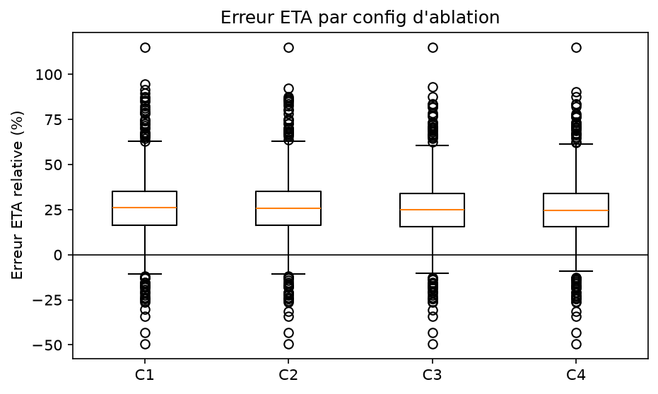
The median bias, by contrast, barely moves across configurations: roughly +0.25 everywhere. Every configuration overestimates transit time by about the same margin; what distinguishes them is the spread around that bias, not the bias itself.
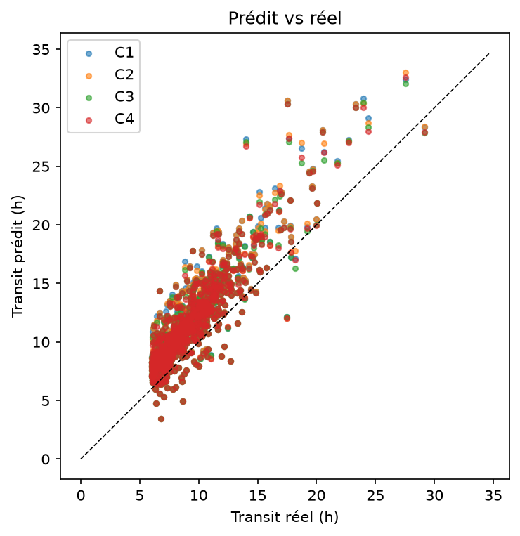
What pays off, measured with a paired bootstrap
A drop in overall MAE does not tell you whether the gap is real or just sampling noise. We test each delta with a paired bootstrap, 10,000 resamples, 95% confidence interval:
- Polar alone (C3 − C1)
- ΔMAE −0.0102, CI [−0.0116, −0.0089] — significant
- Currents alone (C2 − C1)
- ΔMAE −0.0008, CI [−0.0017, +0.0000] — not significant
- Polar + currents (C4 − C1)
- ΔMAE −0.0110, CI [−0.0127, −0.0094] — significant
- Currents added on top of polar (C4 − C3)
- ΔMAE −0.0008 — not significant
The verdict is clear: the AIS-derived speed polar carries the entire measurable gain. CMEMS currents, alone or stacked on top of the polar, produce no effect distinguishable from noise on this sample.
The gain concentrates in rough seas
The overall result hides a heterogeneity that matters for deciding where to invest modeling effort. Breaking MAE down by significant wave height (Hs) band, the AIS polar does almost nothing in flat seas and a great deal in developed seas:
- Hs 0-1 m
- C1 0.2490 vs C3 0.2438 — small gap
- Hs 1-2 m
- C1 0.4086 vs C4 0.3748
- Hs 2-5 m
- C1 0.2923 vs C3 0.2087, C4 0.2018 — widest gap
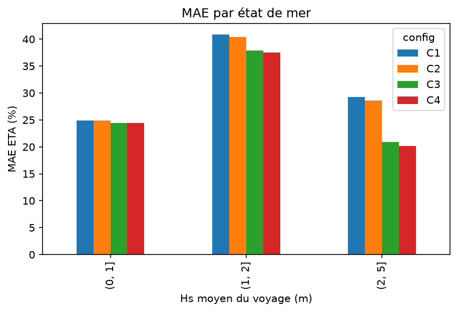
In the 2-5 m bin, the gap between the toy formula and the polar reaches nearly 9 points of MAE. That is exactly the zone where a poorly modeled speed loss costs the most on an arrival schedule — and exactly where the AIS polar delivers the most.
What this validation does not say
A systematic median bias of roughly +25% runs through all four configurations. It is not caused by the physics under test: it comes from the engine itself — a default safety speed-loss factor, and a −1 kn penalty on upwind tacking that triggers on about 62% of legs. That bias needs to be fixed at the engine level, not read as a verdict on currents or the polar.
The sample covers short-to-medium North Sea transits, cargo only; it says nothing about another basin or vessel type. The calm-speed baseline is itself derived from AIS-reported speed through water (STW), an estimate rather than an independent measurement: the study validates weather-driven modulation, not an absolute commercial speed. Finally, a near-zero currents delta means the signal falls below the detection threshold on these specific transits — not that currents never matter, particularly on routes or basins where they are more structuring.
What remains solid: across 800 voyages that actually sailed, the AIS-derived speed polar is the feature that pays, and it pays the most in rough seas — discover SeaRoute-Py, our weather-and-ocean routing engine.
Sources and references
The metrics, comparisons and maps specific to this article are OceanData Consulting results and calculations; the links below document the datasets, standards and publications used.
Facing a similar modeling or metocean data challenge?
From physical model calibration to operational AI post-processing, we help turn marine observations into validated, decision-ready forecasts.
Frequently asked questions
How do you validate a maritime routing ETA prediction?
By replaying real voyages with known actual transit times — here 800 cargo voyages sampled from North Sea AIS history (March-May 2024) — through the routing engine forced with historical weather and ocean conditions (ERA5, CMEMS), then comparing predicted to real transit time voyage by voyage.
Do currents improve ETA accuracy?
On this sample of 800 North Sea voyages, adding CMEMS currents alone produces no effect distinguishable from noise (delta MAE -0.0008, 95% CI including zero). It is the AIS-derived speed polar that carries the measurable gain (delta MAE -0.0102, significant).
Under which sea conditions does the AIS polar deliver the most gain?
The gain concentrates in rough seas: in the Hs 2-5 m bin, the MAE gap between the toy wave formula and the polar reaches nearly 9 points, versus a small gap in flat seas (Hs 0-1 m).