
By Matthieu Caillaud · Founder, oceanographer
A speed-loss formula published in 1980 and five million recent AIS positions agree almost everywhere — and where they disagree, the disagreement is itself informative. Here is how we confronted Kwon's empirical formula, still at the core of commercial routing engines, against speeds actually observed at sea in the North Sea, and why the right engineering answer is not to pick a side but to chain both.
A 1980s formula, still in production
Kwon's formula estimates a vessel's speed loss as a function of sea state: ΔV% = 3.0 × (1.7 − 0.9·Cb) × (180/Lpp) × Hs × direction factor, with the direction factor set to 1.0 for head seas, 0.7 for beam seas, and 0.2 for following seas. Developed forty years ago from tank tests and operational feedback, it remains today what most commercial routing engines use to turn a sea state into a predictable speed over ground.
A formula that old raises a simple question: does it still hold up against data we did not have in 1980 — millions of timestamped AIS positions, per vessel, per real sea state? That is the question we put to our own North Sea traffic data.
Building the ground truth: per-sea-state speed tables from AIS
We built, from raw AIS, median speed-through-water tables for cargo vessels, binned by significant wave height (Hs) and wave incidence angle. Every cell in the table is an observed median, not a physical estimate. Cells resting on fewer than 30 AIS pings are masked — below that threshold, the median is not reliable. The resulting polar is valid up to Hs 5 m; beyond that, observation coverage becomes too sparse to use directly.
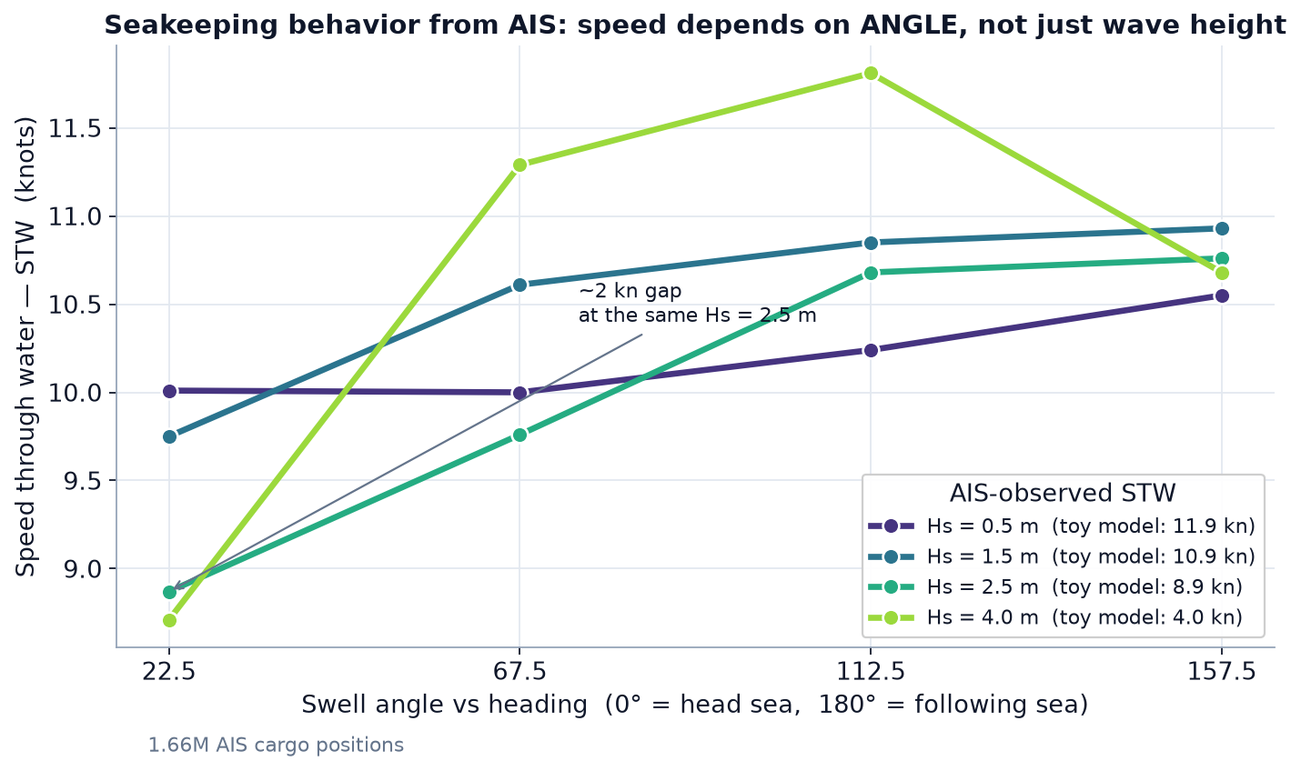
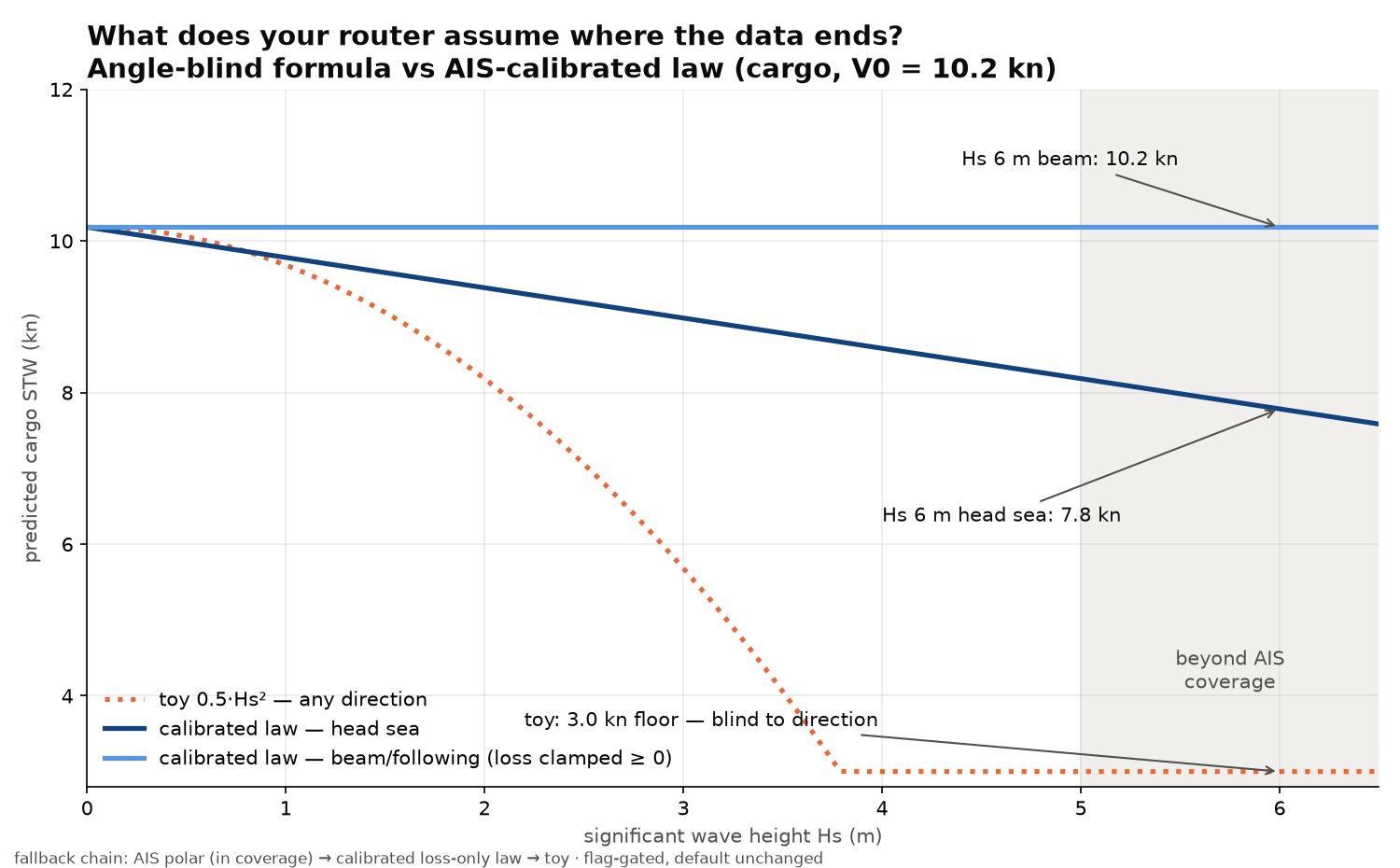
An old internal "toy" formula, 0.5·Hs², gave a rough intuition but collapsed to a 3-knot floor as sea state rose, and ignored incidence angle entirely — head sea and following sea treated identically. Against the AIS polar, it was visibly wrong. We retired it from the production pipeline.
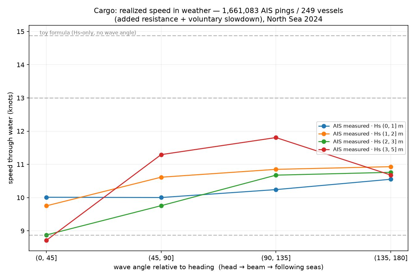
Kwon against AIS: agreement holds in the operational band
We overlaid Kwon's envelope — computed for a fleet block coefficient Cb between 0.60 and 0.85 and a length between perpendiculars Lpp between 120 and 250 m — onto the 16 cells of the AIS polar. 10 of the 16 cells fall inside Kwon's envelope. In the Hs 1.5–2.5 m band, which concentrates most of the observed traffic, Kwon's central curve tracks the AIS medians almost perfectly.
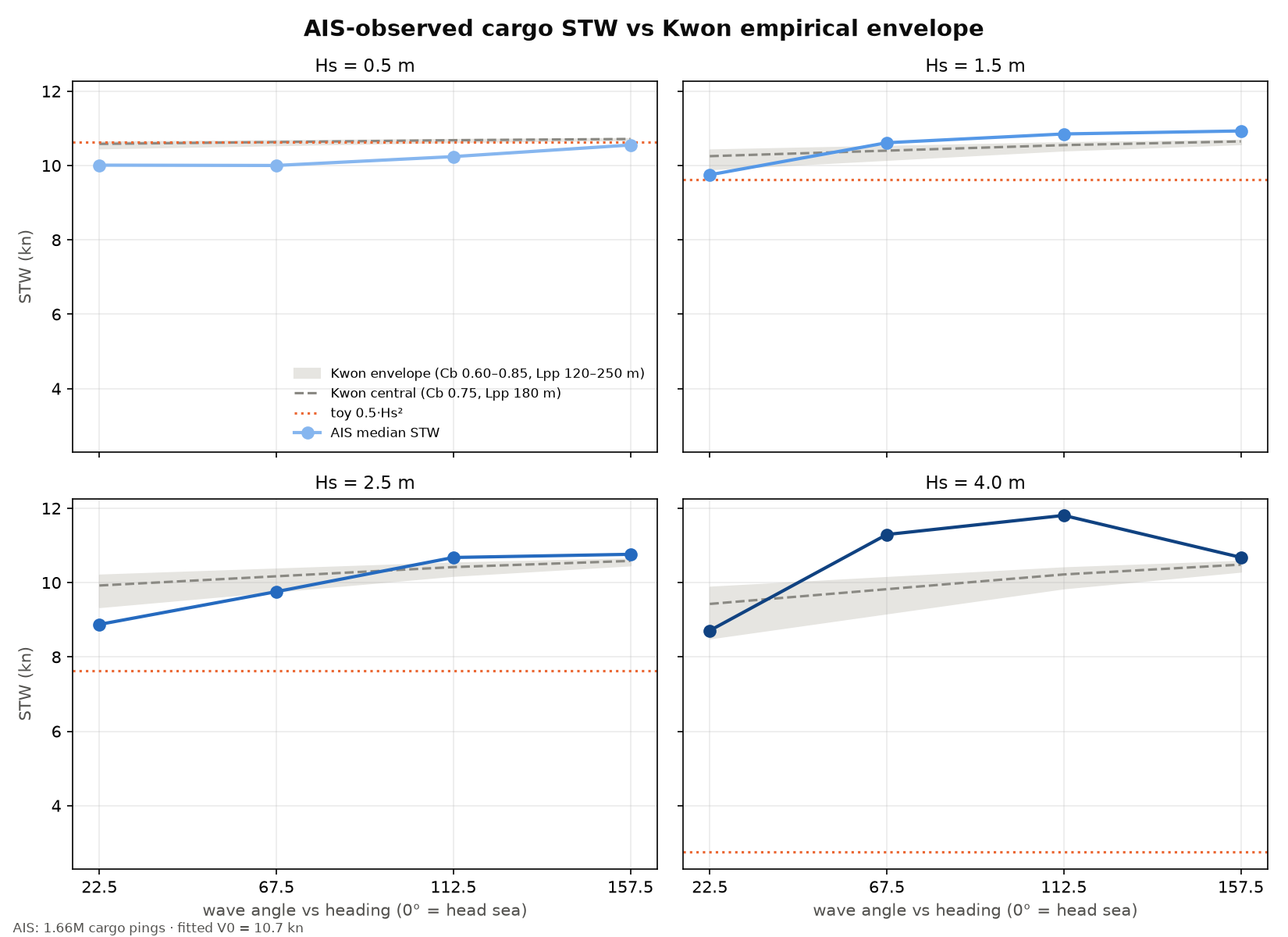
That is a reassuring result, but it is not the conclusion of the exercise. What the overlay mostly reveals is where the agreement breaks down — and why.
Recalibrating the coefficients on five million positions
We then fit Kwon's functional form directly on five million AIS positions per ship class, rather than just comparing the curves visually. This regression validates the model's physics in the operational band and reveals its behavior beyond it.
- Head-sea coefficient — cargo
- k ≈ 3.9%/m of Hs, calibrated on AIS.
- Head-sea coefficient — tanker
- k ≈ 9.1%/m of Hs, calibrated on AIS.
- Direction factor at 67.5°
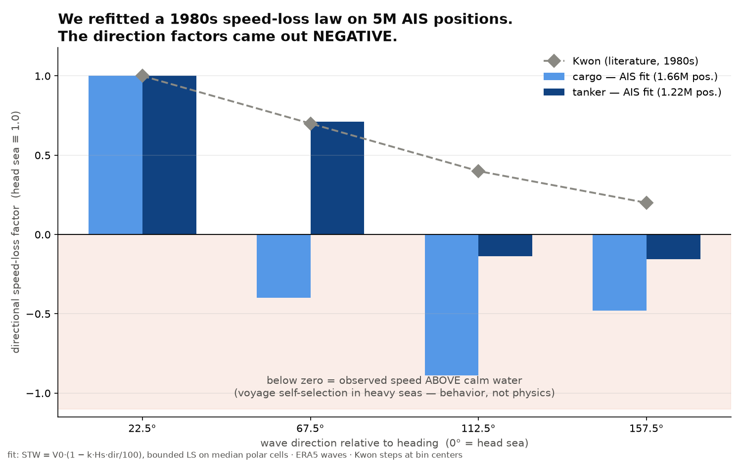
- 0.71 observed versus 0.7 in Kwon’s published literature — validated to the second decimal.
The agreement at 67.5° is the sharpest result of the whole exercise: a factor published in 1980, never recalibrated since, lands within 0.01 of what five million recent North Sea positions actually observe. On this specific point, Kwon's physics has not aged.
What AIS actually measures: not just added resistance
Two anomalies deserve to be surfaced rather than smoothed over, because they say something important about the nature of AIS data itself.
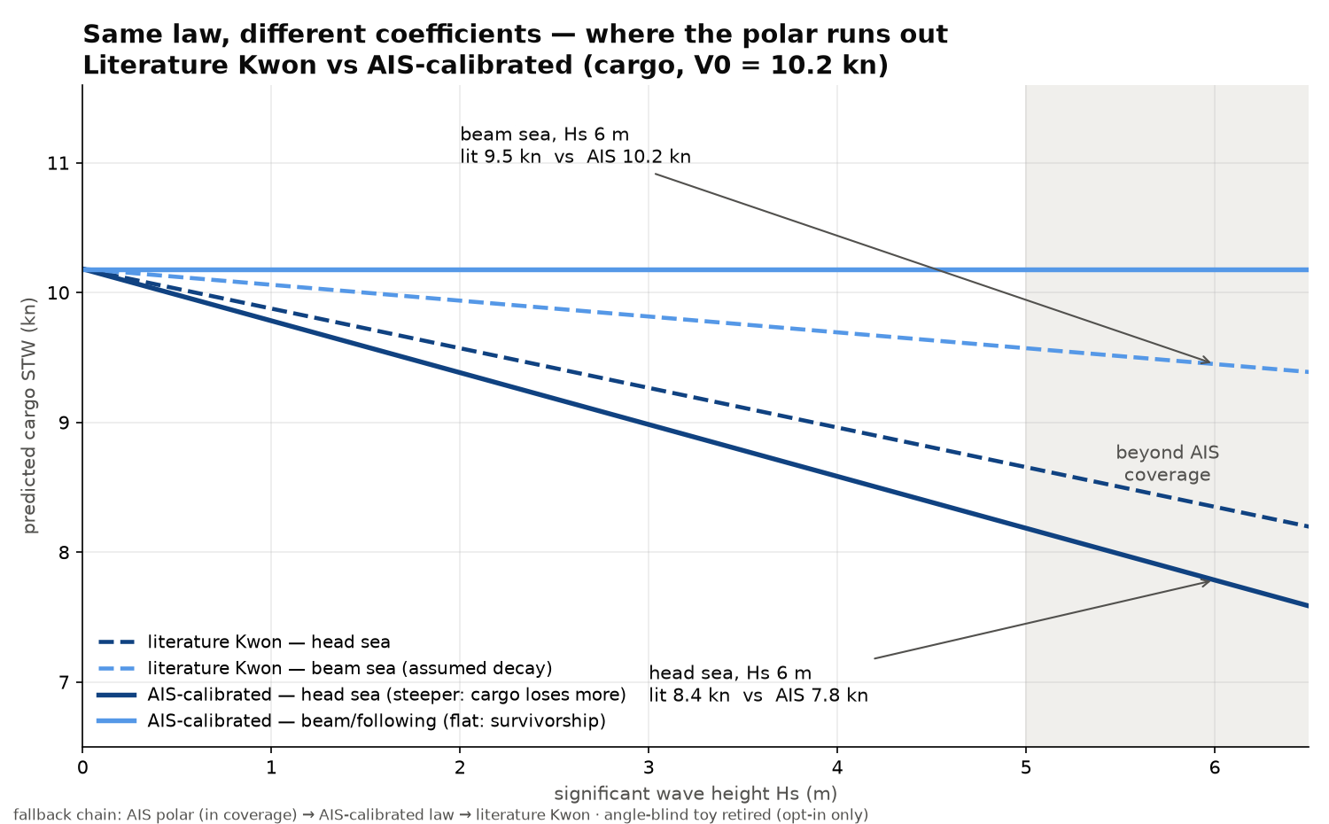
The first: the beam-sea and following-sea direction factors come out negative in the fit. At Hs 4 m in beam or following seas, observed speed-through-water is above calm-water speed. That is not a hydrodynamic effect — it is a survivorship artifact. Only vessels that chose a favorable heading are present in the sample at these sea states; those that would have faced an unfavorable beam sea likely changed course or speed before the measurement captured them. In the production fallback, these factors are clamped to zero rather than left negative.
The second: at Hs 2.5 m in head seas, observed AIS losses exceed what Kwon predicts. Here the data is not capturing added resistance from waves alone — it is also capturing a captain's voluntary slowdown, for cargo comfort or out of caution. AIS structurally mixes involuntary loss with bridge behavior. That is a feature for an ETA prediction, which should reflect what vessels actually do. It is a bias for a pure hydrodynamic study, which is after added resistance alone.
Extrapolating beyond AIS coverage: where Kwon and AIS diverge
Beyond Hs 5 m, AIS cells are masked for lack of sufficient traffic — but the calibrated model can be extrapolated. At Hs 6 m for a cargo vessel, the AIS-calibrated extrapolation gives 7.8 knots in head seas, a 23% loss, against 8.4 knots for literature Kwon. In beam seas the gap runs the other way: 10.2 knots calibrated versus 9.5 knots literature.
These gaps do not lend themselves to direct validation — there simply is not enough commercial traffic at Hs 6 m in the North Sea to confirm them cell by cell. That is precisely why production does not rely on a single model.
The engineering answer: a three-tier fallback, not a dogma
A single model would have forced a choice between two errors: over-generalizing AIS beyond its coverage, or ignoring a real signal in the range where AIS is dense. Production therefore uses a three-tier fallback chain, each tier used in the domain where it is best justified:
- AIS polar directly for Hs ≤ 5 m — the observed median, cell by cell, when traffic density allows it.
- AIS-calibrated Kwon for Hs 5–6 m — Kwon's functional form, with coefficients recalibrated on five million positions.
- Literature Kwon beyond Hs 6 m — the 1980 formula as published, outside any usable observation coverage.
A draft correction rounds out the model, Admiralty-style: factor f = clamp((draft/nominal draft)^(−α), 0.90, 1.15), with a literature α of 0.22, recalibrated on North Sea AIS data with declared draught from spring 2024.
What we do not claim
This calibration carries explicit limits. AIS mixes involuntary loss with captain behavior — an advantage for ETA, a bias for pure hydrodynamics. Heavy sea states suffer from selection bias: only vessels that chose to stay at sea, and often to deviate course, are observed there. A residual non-tidal current bias remains and is region-dependent; these figures hold for the North Sea, spring 2024, not elsewhere without a fresh calibration. Ballast and laden vessels are pooled together — draft is not yet binned in the speed polar. And AIS-declared draught is crew-entered data, often stale.
A formula from 1980 and five million AIS positions agree across most of the operational range. Where they diverge, the divergence is not a calibration failure — it is evidence that captains are not resistance curves. That is the tiered reading, level by level, that we put into production rather than settling on a single model.
Sources and references
The metrics, comparisons and maps specific to this article are OceanData Consulting results and calculations; the links below document the datasets, standards and publications used.
Facing a similar modeling or metocean data challenge?
From physical model calibration to operational AI post-processing, we help turn marine observations into validated, decision-ready forecasts.
Frequently asked questions
What is Kwon’s formula and why is it still used?
It is a 1980 empirical formula estimating a vessel’s speed loss as a function of wave height, block coefficient, length, and incidence direction. It remains the standard in commercial weather routing engines.
Does AIS confirm Kwon’s formula?
Largely yes in the operational band: 10 of 16 AIS cells fall inside Kwon’s envelope, and the direction factor at 67.5° (0.71 observed versus 0.7 in the literature) is validated to the second decimal. Beyond Hs 5 m and in beam or following seas, gaps appear, partly due to selection bias in AIS data.
How does production combine AIS and Kwon’s formula?
Through a three-tier fallback chain: direct AIS polar up to Hs 5 m, AIS-calibrated Kwon between 5 and 6 m, then literature Kwon beyond, complemented by an Admiralty-style draft correction.