
By Matthieu Caillaud · Founder, oceanographer
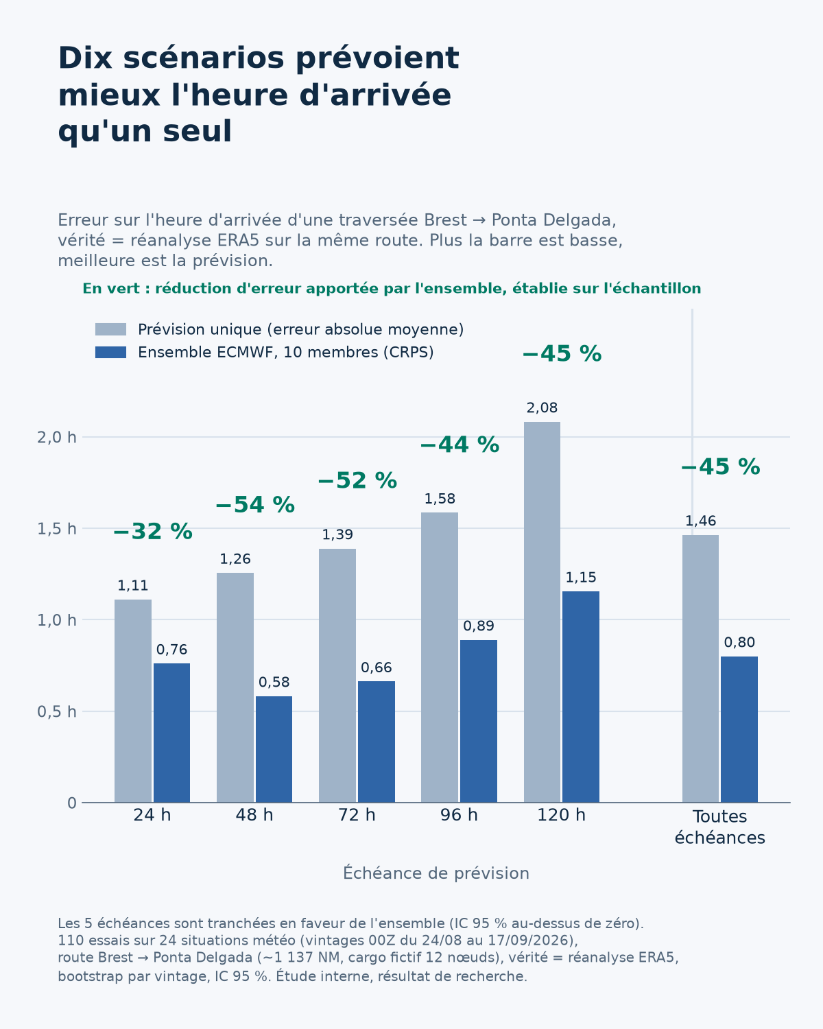
A single weather forecast gives one arrival time; an ensemble forecast gives ten, and shows how far they diverge. We measured what that difference is worth on a four-day crossing, Brest → Ponta Delgada. On arrival time, the gain is clear: the mean error falls from 1 h 36 min with the single forecast to 51 min with the ECMWF ensemble, and the result holds at all five lead times tested, from 24 to 120 h. On route choice, however, the ensemble did no better than a direct route. This article presents both results, because neither makes sense without the other.
The setup: one fixed route, two forecasts, one independent truth
The question is deliberately narrow: for a given route, which forecast predicts the arrival time best? The SeaRoute-Py engine replays the same geometry three times: under the ECMWF deterministic forecast, under 10 of the 50 members of the ECMWF ENS ensemble from the same cycle, and under the ERA5 reanalysis, which serves as the truth. Each member supplies both its wind and its waves, so each replayed trajectory corresponds to a consistent atmosphere-sea state.
- Route
- Brest → Ponta Delgada (São Miguel, Azores), about 1,137 NM, 102.7 h crossing
- Vessel
- fictitious 12-knot cargo ship, identical in every branch
- Departure lead times
- 24, 48, 72, 96 and 120 h after the forecast is issued
- Sample
- 162 trials over 35 distinct weather situations (00Z cycles from 24 August to 28 September 2026)
- Truth
- ERA5/ECWAM reanalysis replayed on the same route, independent of the system under evaluation
- Metrics
- mean absolute error for the single forecast, CRPS for the ensemble, in the same unit (hours)
- Uncertainty
- bootstrap by weather situation, 2,000 resamples, 95 % confidence interval
Two precautions frame the figure. The protocol (lead times, metrics, decision rule) was frozen on 18 September, before the ERA5 truth was even downloaded. And the resampling unit is the weather situation, not the trial: two departures from the same cycle share the same weather, and counting them as independent would artificially tighten the intervals.
The result: the ensemble cuts ETA error by 39 to 53 % depending on lead time
- 24 h
- single forecast 1.17 h, ensemble 0.71 h: gain +38.8 %, 95 % CI [+21.4; +52.2]
- 48 h
- single forecast 1.40 h, ensemble 0.66 h: gain +52.7 %, 95 % CI [+41.4; +61.1]
- 72 h
- single forecast 1.81 h, ensemble 0.86 h: gain +52.5 %, 95 % CI [+38.2; +62.8]
- 96 h
- single forecast 1.73 h, ensemble 1.00 h: gain +42.3 %, 95 % CI [+18.8; +56.9]
- 120 h
- single forecast 2.02 h, ensemble 1.08 h: gain +46.3 %, 95 % CI [+31.5; +58.0]
- All lead times
- single forecast 1.60 h, ensemble 0.85 h: gain +46.9 %, 95 % CI [+37.5; +55.5]
The gain is the CRPSS, the error reduction of the ensemble relative to the single forecast. At all five lead times the confidence interval lies entirely above zero: the ensemble is better, and the sample is large enough to establish it lead time by lead time. At 120 h, the single forecast is off by 2 h 01 min on average, the ensemble by 1 h 05 min.
This verdict was not a given. A first reading, on 18 September, covered only 14 weather situations: the gain was already positive everywhere, but three lead times out of five remained undetermined, their interval touching zero. The protocol provided for rerunning the measurement as the archive grows, changing nothing else. The 28 September rerun added ten weather situations, and the three lead times tipped over. No sign reversed between the two readings: it is the intervals that tightened. Before the rerun, the initial cohort was replayed on the current version of the engine and returned the same values bit for bit, which rules out a software-version effect.
The figures above come from a second rerun, on 9 October: the ERA5 truth is extended to 4 October, which adds eleven late-September situations. The 35 situations include the 24 of the 28 September reading; this is an updated reading on a larger sample, not an independent test. All five lead times still favour the ensemble, no sign reverses, and the 110 trials common to both readings return the same values on the current version of the engine. The mean error rises on both sides, from 1 h 28 min to 1 h 36 min for the single forecast and from 48 to 51 min for the ensemble, because the added situations are harder: the single forecast is off by 2.10 h on average there, against 1.43 h on the original 24 situations, where ten trials still pending on 28 September are now evaluated. The relative gain stays of the same order.
What the ensemble does not correct
A better ensemble is not a calibrated ensemble. Two limits remain, measured on the same sample, and they matter for how the forecast is used.
- The range is too narrow at short lead times. With 10 members, the interval between the 10th and 90th percentiles should contain the truth in about 65.5 % of cases. At 24 h it contains it in only 51 % of cases; at lead times of 48 to 120 h, in 67 to 71 % of cases, and in 65 % across all lead times. Short-lead underdispersion also appears, mixed with a bias, when the ensemble's wind and waves are compared directly with satellite observations.
- A systematic delay remains. On average, the ensemble announces an arrival 0.81 h later than the truth, the single forecast 0.73 h. The ensemble reduces the spread of the error, not this shared bias: its mean is even slightly later than the single forecast at lead times of 24 to 72 h, slightly less so at 96 and 120 h. This bias calls for a separate recalibration.
And for choosing the route? The result is unfavourable, and we publish it
Predicting the arrival time better on a fixed route says nothing about the value of the ensemble for choosing the route. We tested that separately, on 13 crossings of the same corridor, with protocols frozen before the first computation. For each situation, an A* is run under the single forecast, an A* under each of the 10 members, and a "robust" route is then selected by penalising unfavourable scenarios. The routes are then replayed under ERA5.
- Robust route versus deterministic route
- arrival 1.90 h earlier, 95 % CI [−2.99; −1.04], modelled fuel −2.43 %
- Direct route versus robust route
- arrival 4.87 h earlier, 95 % CI [−8.05; −2.05], modelled fuel −8.19 %
The first figure looks favourable to the ensemble, but its decomposition reclassifies it: the ETA difference follows the distance difference almost exactly (correlation 0.95). The robust route wins because it is shorter; the ensemble does not read the weather better, it prevents betting on a detour that the single forecast judged profitable. Hence the second test, against a direct route: the great circle, with a single waypoint to go around São Miguel. It arrives 4.87 h earlier than the robust route. At equal distance, routing does gain about 1.2 h, but it pays about 6.1 h of detour to get it.
This result has limits that we state alongside it. The 13 crossings took place in rather manageable seas, with a maximum significant wave height of 3.9 m across the whole cohort, which is the regime in which a detour has the least reason to pay. The direct route underwent no seakeeping check, and the bathymetric check was inactive on all three branches. The share of the 73 NM of detour attributable to the A* grid rather than to a weather-driven choice was not measured. Fuel is modelled, on an uncalibrated vessel profile. And an open-ocean corridor, with no strait or dominant current, does not transfer to other routes. But on this corridor and over this period, the finding is clear: the ensemble did not save time by choosing the route.
On a short crossing, the range is no longer enough
The same exercise, this time compared with arrivals actually observed, covered 801 AIS voyages between Ushant and the Pas-de-Calais. The ensemble remains better than the single forecast there, but only slightly: +3.5 %, 95 % CI [+2.2; +5.2]. Its range is 11 minutes wide for an actual error of about 2 hours: on a one-day crossing, the spread of the weather scenarios falls far short of covering the gap observed at arrival. The sources of this residual gap are not identified by this study. The contrast with the long crossing, where the members have time to diverge, is however clear.
What to take away
On a long crossing, the ensemble forecast is a better instrument for announcing an arrival time: 51 minutes of mean error instead of 1 h 36 min, established at all five lead times tested. This is directly useful information for planning a port call, a berth slot or a contractual window. It is not a promise of a faster route: on the tested corridor, the direct route beat routing, with or without an ensemble.
What this study does not say: it covers a fictitious vessel and a single corridor, on late-summer situations only; its truth is a preliminary ERA5 reanalysis (ERA5T), not an observed arrival time; and the ensemble range remains too narrow at 24 h. It is an internal research result, which will be rerun as the archive covers autumn and winter.
The replay method is described in our replay of 800 AIS voyages, and an openly negative first verdict on routing gain appears in the retro-routing audit. The engine is presented on the SeaRoute-Py page.
Sources and references
The metrics, comparisons and maps specific to this article are OceanData Consulting results and calculations; the links below document the datasets, standards and publications used.
Facing a similar modeling or metocean data challenge?
From physical model calibration to operational AI post-processing, we help turn marine observations into validated, decision-ready forecasts.
Frequently asked questions
What does an ensemble forecast gain on a ship’s arrival time?
On a 102.7 h Brest to Ponta Delgada crossing, replayed under 162 departures from 35 weather situations and checked against the ERA5 reanalysis, 10 members of the ECMWF ensemble bring the mean ETA error from 1.60 h (single forecast) down to 0.85 h, a gain of 46.9 %, 95 % CI [+37.5; +55.5]. The gain is established separately at all five departure lead times, from 24 to 120 h.
Does routing with the ensemble save time?
Not on the tested corridor. Over 13 crossings, the robust ensemble route arrives 1.90 h earlier than the deterministic route, but only because it is shorter; a direct route still arrives 4.87 h earlier, 95 % CI [−8.05; −2.05]. The cohort saw manageable seas (maximum Hs 3.9 m), and the result does not transfer to another corridor.
Is the range given by the ensemble reliable?
Not yet at short lead times. With 10 members, the P10–P90 interval should contain the truth in about 65.5 % of cases; it does so in only 51 % of cases at 24 h, against 65 % across all lead times. A systematic delay shared by the ensemble and the single forecast also remains: 0.81 h for the ensemble mean, 0.73 h for the single forecast.